What This Article Covers
- Why a second solver: Why a second, independent Boltzmann solver (MultiBolt) was added as a cross-check alongside LoKI-B-cpp.
- Coverage gained: What this campaign adds relative to Campaign 1 (see the metrics and phase table below).
- What the comparison revealed: Where the two solvers agree, where they disagree, and what is still open.
← See the original V&V methodology (Campaign 1)
Why Cross-Validate Against a Second Solver?
A global model's answer is only as good as its electron energy distribution function (EEDF), and the EEDF comes from a Boltzmann solver. Every Boltzmann solver makes choices: two-term or multi-term expansion, how ionization growth is renormalised, how "effective" cross sections are reduced to elastic ones. With a single solver, those choices are invisible. A residual against Dias et al. (2023) could come from the global-model kinetics or from the EEDF, and there is no way to tell which.
Campaign 2 therefore put a second, independently developed solver, MultiBolt (Texas Tech, multi-term), behind the same interface as LoKI-B (IST Lisbon, two-term). Where the two agree, confidence goes up. Where they disagree, there is a precise question to chase.
Key Insight
A second solver is a measuring instrument. Integrating MultiBolt surfaced seven defects, including a sign-flipped elastic-loss term reached through "effective" cross sections. Cross-checking the coupled sweeps found four more, one of them only because MultiBolt N=2 and N=10 showed the same offset. Comparing a single solver against experiment would not have found them.
Verification: Adding MultiBolt as a Second EEDF Ground Truth
MultiBolt was added as an alternative EEDF backend: the global-model solver stays backend-agnostic, and all backend-specific logic lives in one wrapper that translates the setup, runs the solver and parses its output. Verification then went from easy cases to hard ones:
- Argon (single ground state, no vibrational manifold) — 0.1–2 % agreement with LoKI-B on the swarm parameters from 50 to 2000 Td, after fixing a units bug in the output parser.
- O$_2$ at fixed E/N (molecular, vibrationally active, attaching) — started at 2.6× on electron temperature. After the "effective" cross-section defect was found and fixed, $T_e$ agreed to 1–3 %, mobility to < 0.5 %, and the main inelastic rate coefficients to ~1 % at 40–300 Td.
- Coupled O$_2$ discharge — the full 12-point sweep with LoKI-B, MultiBolt N=2 and MultiBolt N=10.
Each defect was chased the same way: change one input at a time until the discrepancy moves, then read the few lines of solver source that change points to. For example, swapping only the O$_2$ momentum-transfer cross section from EFFECTIVE to ELASTIC collapsed a 2.7× discrepancy to 1.00×.
Validation: What the Cross-Solver Comparison Shows
The coupled sweeps are where the two solvers earned their keep. Early sweeps had MultiBolt N=10 needing 10–23 % more field than LoKI-B and both solvers overpopulating O$_2$(X, v=1) by up to 8.7×. Each was traced to the coupling, not the solvers: O$_2$(X) was counted twice, the vibrational rates were frozen at the wrong temperature, MultiBolt was solving a different Boltzmann problem from LoKI-B, and three reactions silently got no rate on the MultiBolt path. With these fixed, all 36 pressure points were run again for the results below.
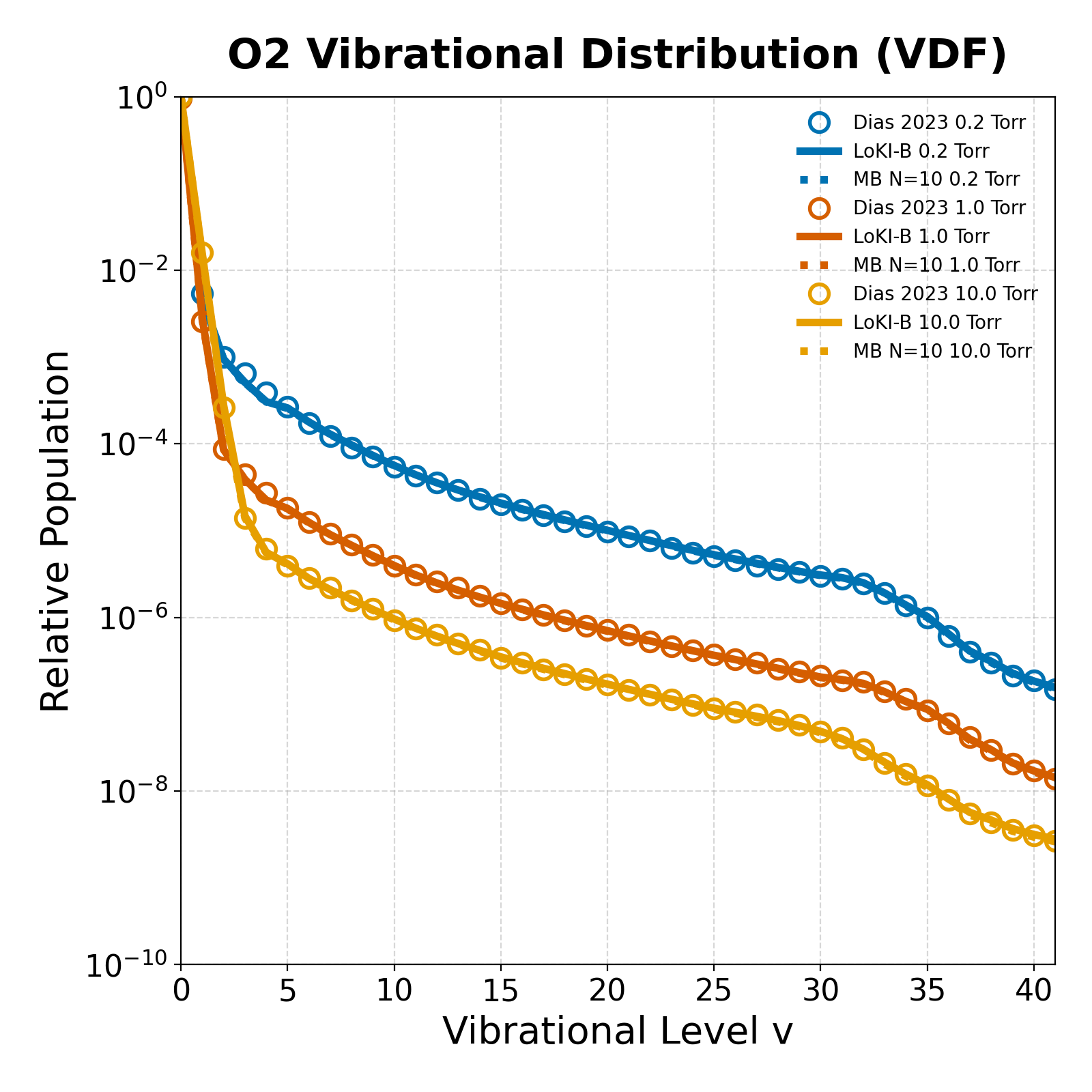
With LoKI-B, pyFrost-GM now reproduces Dias et al. (2023) to a mean of 0.9 % in E/N, 0.3 % in gas temperature and 1.8 % in O($^3$P) and O$_2(a^1\Delta_g)$, and the v=1/v=0 ratio is within 12 % of the paper's Fig. 15. MultiBolt N=2, given the same Boltzmann problem, agrees with LoKI-B to within 0.5 % at every pressure. MultiBolt N=10 then isolates the multi-term effect: 1.7–4.3 % less field and 2–4 % less O($^3$P) than N=2.
One residual is common to all three solvers: at 0.19 Torr, O$_2(a^1\Delta_g)$ is 14 % low and E/N 3.8 % high. Because it does not depend on the solver, it points at the chemistry and is carried into Campaign 3. The O($^3$P) pathway plots now count O atoms (O($^3$P) + O($^1$D)) and normalise over all sources, as the paper's Fig. 14a does.
Coverage: Before vs. After This Iteration
The validation targets are unchanged: 2 publications and 7 reproduced figures (6 from Dias et al. 2023, plus electron density from Alves et al. 2026). What grew is the depth. Every figure is now produced by three EEDF configurations (LoKI-B, MultiBolt N=2, MultiBolt N=10), and with excited-state populations fed back into the EEDF.
Iteration Timeline
Campaign 2 ran from 2 to 29 September 2026: the integration work from 2 to 20 September, the first sweeps up to 23 September, and on 28–29 September the coupling fixes, the speed-up and the final sweeps.
| Phase | Dates | Commits | What Happened |
|---|---|---|---|
| 1. Wire in MultiBolt | Sep 2–3 | 4 | LXCat cross sections extrapolated to 10 keV for high-E/N convergence; MultiBolt as an alternative EEDF backend with its own power-balance calculation; LXCat ingestion fixes for LoKI-B; integration rules recorded for later sessions |
| 2. O₂ Parity | Sep 9–10 | 9 | Per-vibrational-level pseudo-species; EFFECTIVE→ELASTIC fix; bracket-then-Brent E/N search; N₂ rate-binding regression fixed; integration case study written |
| 3. Feedback & Speed | Sep 14 | 4 | Reversible-process key fix; energy-grid carry-forward (2.3× faster; lost in a refactor the next day and restored on 29 September); excited-state feedback made the default for the Dias case; discrepancy investigation documented |
| 4. State Mapping & Sweeps | Sep 15–23 | 11 | Electronic-state mapping and fraction normalisation for MultiBolt; metastable and detachment process strings; v = 0 exclusion; first LoKI-B, N=2 and N=10 sweeps |
| 5. Coupling Fixes & Final Sweeps | Sep 28–29 | 16 | O₂(X) double count fixed; vibrational rates refreshed at each restart; MultiBolt given LoKI-B’s Boltzmann problem, all rates integrated over the EEDF as in LoKI-GM; three reactions bound on the MultiBolt path; profiling-led speed-up (4.4× per pressure point) checked against a frozen reference; all 36 points rerun |
The AI-Agentic Workflow, Campaign 2
The workflow from Campaign 1 carried over, with two changes. Integration rules and findings were written into the repository (a MultiBolt ruleset, an integration case study and a discrepancy investigation plan), so every new session starts from what is already known instead of from memory. And investigation tasks were matched to model capability: mechanical extraction to smaller models, cross-language semantics and physics causality to the strongest one.
Where AI Helped
- Adapter and preprocessing code: translating the setup into MultiBolt's inputs, parsing its outputs, and rewriting LXCat files (retagging, EFFECTIVE→ELASTIC).
- Bisection experiments: running the one-variable-at-a-time comparisons that localised each defect.
- Evidence extraction: pulling every quoted number from output files, including the check that showed the N=2 and N=10 sweeps ran on different code versions.
Where Physics Expertise Was Essential
- Choosing falsifying tests: ruling out dissociative attachment (0.2 % of the power balance) and continuous rotational cooling (Te 2.148 → 2.149 eV) before suspecting the cross sections.
- Reading the coupled result: at fixed current, $n_e \propto 1/v_{drift}$, so an electron-density excess and a reduced-field deficit are the same error, not two.
- Deciding what counts as evidence: one AI-reported "improvement" in $n_e$ turned out to be an artifact. The "before" run already contained the fix, as byte-identical output files showed. The rules that followed: verify that a "before" really is before, change one variable at a time, and quote numbers from files on disk.
Physicist-in-the-Loop
With two solvers, the physicist's job shifts from checking one answer to deciding which disagreement to chase, and which piece of evidence is strong enough to act on. The AI runs the experiments; the physicist decides what an experiment has actually shown.
What This Unlocks
A second, independent EEDF solver behind the same interface turns solver choice into a variable that can be tested:
- Solver-independent conclusions — a result that holds with both LoKI-B and MultiBolt does not depend on one code's assumptions.
- Multi-term physics where it matters — above ~250 Td the two-term and multi-term mobilities begin to diverge (−6 % at 700 Td, −9 % at 2000 Td), the regime of nanosecond-pulsed discharges.
- A regression net for the whole model — the parity tests caught an N$_2$ rate-binding regression that had nothing to do with MultiBolt.
- Risk mitigation — the model is no longer locked to a single solver's choices or maintenance.
Want to build a validated, cloud-ready version of your scientific code?
Whether it's translating MATLAB/Fortran to Python, setting up automated V&V pipelines, or adopting AI-agentic workflows for your own simulation tools — I can help build the auditable, extensible architecture you need.
Contact for a ConsultationBibliography
- [1] Dias T C et al, "A reaction mechanism for oxygen plasmas" 2023 Plasma Sources Sci. Technol. 32 084003. DOI: 10.1088/1361-6595/aceaa4 — The primary validation benchmark for pyFrost-GM oxygen chemistry.
- [2] Alves L L et al, "LoKI-GM: a global model tool for plasma chemistry studies" 2026 Plasma Sources Sci. Technol. (in preparation). DOI: 10.48550/arXiv.2607.27234
- [2b] Stephens J, "A multi-term Boltzmann equation benchmark of electron-argon cross-sections for use in low temperature plasma models" 2018 J. Phys. D: Appl. Phys. 51 125203. DOI: 10.1088/1361-6463/aaaf8b — MultiBolt
- [3] LoKI-GM — Official MATLAB repository (IST Lisbon)
- [4] Tejero A et al, "The LisbOn KInetics Boltzmann solver" 2019 Plasma Sources Sci. Technol. 28 043001. DOI: 10.1088/1361-6595/ab0537 (Open Access)